3dgs real-time radiance rendering

introduce 3D Gaussians as a flexible and expressive scene representation.
input:
- cameras calibrated with Structure-from-Motion(SfM)
- initalize the set of 3D Gaussians with the sparse point cloud produced for free as part of the SfM process.
  (only SfM points as input)
optimization of the properities of the 3D Gaussians - 3D position, opacity $\alpha$ (?), anisotropic covarianice, and SH coefficients - interleaved with adaptive density control steps, where we add and occasionally remove 3D Gaussians during optimization

produce （reasonably compact,unstructured,and precise representation of the scene）

real-time rendering solution that uses fast GPU sorting algorithms ansd is inspired by tile-based rasterization. (visibility-aware, allows anisotropic splatting and fast back-propagation(反向传播) to achieve high-quality novel view synthesis)

light field (光场)

The first novel-view synthesis approaches were based on light fields.
SfM estimates a sparse point cloud during camera calibration.
Rendering using volumetric ray-marching has a significant cost due to the large number of samples required to query the volume.

recent methods have focused on faster training and/or rendering mostly by expoiting(开发) three design choices:

the use of spatial data structures to store (neural) features that are subsequently interpolated during volumetric ray-matching
different encoding
MLP capacity

Many methods has limits:

struggle to represent empty space effectively,depending in part on the scene/capture type
image quality is limited in large part by the choice of the structured grids used for acceleration, and rendering speed is hindered(阻碍) by the need to query many samples for a given ray-marching step.

aliasing(走样)
image formation model(成像模型)

Point-based alpha-blending and NeRF-style volumetric rendering

The color C is given by volumetric rendering along a ray:(?)

A typical neutral point-based approach computes the color C of a pixel by blending N order points overlapping the pixel:(?)

–> Points are an unstructured,discrete representation that is flexible enough to allow creation,destruction,and displacement of geometry similar to NeRF.
–> This is achieved by optimizing opacity(?什么意思) and positions.

–> optimization of anisotropic covariance, interleaved optimization/density control, and efficient depth sorting for rendering allow us to handle complete, complex scenes including background, both indoors and outdoors and with large depth complexity.

OVERVIEW

The input to our method is a set of images of a static scene, together with the corresponding cameras calibrated by SfM [Schönberger and Frahm 2016] which produces a sparse point cloud as a side effect. From these points we create a set of 3D Gaussians (Sec. 4), defined by a position (mean), covariance matrix and opacity 𝛼, that allows a very flexible optimization regime.
This results in a reasonably compact(简化) representation of the 3D scene, in part because highly anisotropic volumetric splats(高度各向异性的体积斑点) can be used to represent fine structures compactly. The directional appearance component (color) of the radiance field is represented via spherical harmonics (SH), following standard practice [Fridovich-Keil and Yu et al. 2022; Müller et al. 2022].
Our algorithm proceeds to create the radiance field representation (Sec. 5) via a sequence of optimization steps of 3D Gaussian parameters, i.e., position, covariance, 𝛼 and SH coefficients interleaved with operations for adaptive control of the Gaussian density.
The key to the efficiency of our method is our tile-based rasterizer (Sec. 6) that allows 𝛼-blending of anisotropic splats, respecting visibility order thanks to fast sorting.
Out fast rasterizer also includes a fast backward pass by tracking accumulated 𝛼 values, without a limit on the number of Gaussians that can receive gradients. The overview of our method is illustrated in Fig. 2.

input : a set of images of a static scene + the corresponding cameras calibrated by SfM (produces a sparse point cloud [side effect?]) -> 3D Gaussians (include a position(mean), covariance matrix and opacity alpha)

compact representation of the 3D scene
SH -> The directional appearance component(color) of the radiance field

optimization regime(?)

Model the geometry as a set of 3D Gaussians that don’t require normals.

affine(仿射)

推公式：
3D Gaussian表示了一个三维数据组，满足三维的高斯分布，经过推导之后可以用协方差矩阵的逆和协方差矩阵的行列式表示。
数据需要经过Camera Calibration,所以协方差矩阵也要经过相应的变换，方法是左乘W(世界坐标系到摄像机坐标系的变换矩阵)和J(3D摄像机坐标系到2D像素坐标系的jacobian matrix，为了抵消非线性变换带来的影响)，由于是分布变换，所以还要右乘对应的矩阵的转置。
协方差矩阵经过特征值分解的特征向量和特征值矩阵，在几何意义上是旋转矩阵和缩放矩阵的平方(因为是方差)的形式对应，用V表示旋转矩阵，用L表示特征值矩阵有:

\sum = VLV^{-1}

在论文中用 R 表示旋转矩阵用 S 表示缩放矩阵，则有：

\sum = RSSR^{-1}

用 T 表示变换矩阵，则可以写成：

\sum = RSS^{T}R^{T} = RS(SR)^{T} = TT^{T}

此外，为了节约计算量，使用四元数表示旋转矩阵

covariance matrices have physical meaning only when they are positive semi-definite. --> cannot directly optimize the covariance matrix $\sum$ to obtain 3D Gaussians that represent the radiance field.

constrain(约束)

So, use the formula :

\sum = RSS^{T}R^{T} = RS(SR)^{T} = TT^{T}

And store them separately :

a 3D vector $s$ for scaling
a quaternion $q$ to represent rotation

derive the gradients for all parameters explicitly --> avoid significant overhead due to automatic differentiation during training.

optimization: positions $p$ , $\alpha$ ,covarivance $\sum$ ,SH coefficients

The optimization of these parameters is interleaved with steps that control the density of the Gaussians to better represent the scene.

Inevitably, geometry may be incorrectly palced due to the ambiguities of 3D to 2D projection. --> our optimization thus needs to be able to create geometry and also destroy or mobe geometry if it is incorrect.

The quality of the parameters of the covarivances of the 3D Gaussians is critical. --> large homogeneous areas can be captured with a small number of large anisotropic Gaussians.

Stochastic Gradient Descent

sigmoid activation function for $\alpha$

exponential activation function for the scale of the covariance

Reason : to constrain it in the [0 - 1) range and obtain smooth gradients.

densify every 100 iterations and remove any Gaussians that are essentially transparent.

densify Gaussians with an average magnitude of view-space position gradients above a threshold $\tau_{pos}$

under-reconstructed regions – regions with missing geometric features

over-reconstructed regions – regions where Gaussians cover large area in the scene.

cover the new geometry that must be created (For small Gaussian that are in under-reconstructed regions) --> clone the gaussians. simply creating a copy of the same size, and moving it in the direction of the positional gradient

large Gaussians in regions with high variance need to be split into smaller Gaussians, also initialize their position by using the original 3D Gaussian as a PDF for sampling.

A effective way to moderate the increase in the number of Gaussians is to set the $\alpha$ value close to zero every N = 3000 iterations

Our fast rasterizer allows efficient backpropagation over an arbitrary number of blended Gaussians with low additional memory consumption, requiring only a constant overhead per pixel.

Specially, we only keep Gaussians with a 99% confidence interval intersecting the view frustum. Additionally, we use a guard band to trivially reject Gaussians at extreme positions.

instantiate each Gaussian according to the number of tiles they overlap and assign each instance a key that combines view space depth and tile ID.
sort Gaussians based on these keys using a single fast GPU Radix Sort. ( $\alpha$ blending)
these approximations become negligible as splats approach the size of individual pixels.

During rasterization, the saturation of $\alpha$ is the only stopping cirterion.

During the backward pass, we must therefore recover the full sequence of blended points per-pixel in the forward pass.

traverse the per-tile lists again.

To facilitate gradient computation, we now traverse them back-to-front.

Rasterization

The traversal starts from the last point that affected any pixel in the tile, and loading of points into shared memory again happens collaboratively.
Additionally, each pixel will only start overlap testing and processing of points if their depth is lower than or equal to the depth of the last point that contributed to its color during the forward pass. (深度测试?)
recover intermediate opacities by storing only the total accumulated opacity at the end of the forward pass.
Specifically, each point stores the final accumulated opacity $\alpha$ in the forward process.
We divide this by each point’s $\alpha$ in our back-to-front traversal to obtain the required coefficients for gradient computation.

implementation

SH coefficient optimization is sensitive to the lack of angular information.

optimizing only the zero-order component, and then introduce one band of the SH after every 1000 interations unitl all 4 bands of SH are represented.

Initialization with SfM points helps
Densification
- splitting big Gaussians is important to allow good reconstruction of the background
- cloning the small Gaussians instead of splitting them allows for a better and faster convergence especially when thin structures appear in the scene.
Unlimited is better. If we limit the number of points that receive gradients, the effect on visual quality is significant.
The use of anisotropic volumetric splats enables modelling of fine structures and has a significant impact on visual quality.
spherical harmonics improves (?)

limitations

popping artifacts when our optimization creates large Gaussians

view-dependent appearance
reason: trivial rejection of Gaussians via a guard band in the rasterizer
simple visibility algorithm,which can lead to Gaussians suddenly switching depth/blending order (antialiasing)
do not apply any regularization(正则化) to our optimization
the GPU memory figure could be significantly reduced by a careful low-level implementation of the optimization logic. (i.e. Compression techniques method)

可微的3D Gaussian Splatting

初始化利用SfM的点云，包含 Position(Mean)、Covariance Matrix、Opacity $\alpha$ 、Spherical harmonics

其中：

点的位置(也即3D Gaussian的均值)、
协方差矩阵，决定Gaussian形状
不透明度，用于渲染，把他点往图像平面上投的时候，它们的扩散痕迹是通过这个不透明度，叠加在一起的
球谐函数，用来拟合视角相关的外观（球谐函数本身就是用一组正交基的线性组合来拟合光场）
3D Gaussian，需要一种图元，能够在拥有场景表达能力的时候可微，且显式地支持快速渲染
3D Gaussian点云里面的参数可以在迭代优化的过程中更新，而且能够很容易地用splat的方法，来投影到2D图像上，做非常快的 $\alpha$ 混合（rendering）

Jacobian Matrix的推导

投影公式
投影公式用于将三维空间中的点 $(x, y, z)$ 映射到二维屏幕平面上的点 $(x', y')$ 。

(1)相机坐标系与视图坐标系
首先假设点 $(x, y, z)$ 是在相机坐标系下的三维坐标。相机位于原点，视线沿 $z$ -轴正方向。

$( x, y, z )$ 表示点的三维位置。
$z$ 是点与相机的距离。

(2)转换到投影平面(深度透视)
在相机的投影模型中，投影平面通常设置为距离相机原点为 1 的位置（即 $z = 1$ )。通过投影，三维点 $(x, y, z)$ 会映射到投影平面上的点 $(x_p, y_p, 1)$ ，投影关系为：

x_p = \frac{x}{z}, \quad y_p = \frac{y}{z}

其中：

x/z 表示水平视角下点的位置与深度的比例。
y/z 表示垂直视角下点的位置与深度的比例。

为了将投影平面的坐标 $(x_p, y_p)$ 转换为屏幕上的像素坐标，需要考虑相机的焦距 $f_x$ 和 $f_y$ （单位像素），以及屏幕的分辨率和尺度变换。投影公式为：

x' = f_x \cdot x_p = \frac{f_x \cdot x}{z}, \quad y' = f_y \cdot y_p = \frac{f_y \cdot y}{z}

其中：

f_x = \frac{\text{Width}}{2 \cdot \tan(\text{水平视角FovX} / 2)}

f_y = \frac{\text{Height}}{2 \cdot \tan(\text{垂直视角FovY} / 2)}

其中 $f_x, f_y$ 是相机内参，定义了投影比例。

结合以上推导，透视投影公式可以写为：

x' = \frac{f_x \cdot x}{z}, \quad y' = \frac{f_y \cdot y}{z}

推导Jacobian矩阵

在计算机图形学和3D变换中，Jacobian 矩阵用于描述从一个空间（例如世界坐标系）到另一个空间（例如视图空间或屏幕空间）的坐标映射变化率。在这个例子中，Jacobian 矩阵 J 描述从 3D 视图空间到 2D 投影空间（屏幕坐标）的变化。

Jacobian 矩阵是投影变换对输入坐标的偏导数矩阵：

J = \frac{\partial(x', y')}{\partial(x, y, z)}

它表示投影变换中，每个 3D 坐标分量的微小变化对 2D 坐标的影响。

将以上偏导数写成矩阵形式：

J = \begin{bmatrix} \frac{\partial x'}{\partial x} & \frac{\partial x'}{\partial y} & \frac{\partial x'}{\partial z} \\ \frac{\partial y'}{\partial x} & \frac{\partial y'}{\partial y} & \frac{\partial y'}{\partial z} \end{bmatrix} = \begin{bmatrix} \frac{f_x}{z} & 0 & -\frac{f_x \cdot x}{z^2} \\ 0 & \frac{f_y}{z} & -\frac{f_y \cdot y}{z^2} \end{bmatrix}

glm::mat3 J = glm::mat3(
    focal_x / t.z, 0.0f, -(focal_x * t.x) / (t.z * t.z),
    0.0f, focal_y / t.z, -(focal_y * t.y) / (t.z * t.z),
    0, 0, 0);

这个矩阵用在后续的高斯分布投影中，用来减轻非线性变换对视图带来的影响

协方差矩阵转换为几何表达的椭圆

在二维高斯分布中，等概率密度的轮廓是一个椭圆，其定义如下：

(x - \mu)^T \Sigma^{-1} (x - \mu) = c

其中把 $(x-\mu)$ 当作向量基，协方差矩阵的逆矩阵看作基的系数，可以转化为一个xy坐标系上面的二次曲线

我们将椭圆的隐式方程由协方差逆矩阵 $\Sigma^{-1}$ 给出：

[x \; y] \begin{bmatrix} \Sigma^{-1}_{11} & \Sigma^{-1}_{12} \\ \Sigma^{-1}_{12} & \Sigma^{-1}_{22} \end{bmatrix} \begin{bmatrix} x \\ y \end{bmatrix} = 1

展开后：

\Sigma^{-1}_{11} \cdot x^2 + 2 \cdot \Sigma^{-1}_{12} \cdot xy + \Sigma^{-1}_{22} \cdot y^2 = 1

我们知道对称矩阵协方差矩阵为：

\Sigma = \begin{bmatrix} \text{cov.x} & \text{cov.y} \\ \text{cov.y} & \text{cov.z} \end{bmatrix}

其逆矩阵 $\Sigma^{-1}$ ：

\Sigma^{-1} = \frac{1}{\det(\Sigma)} \begin{bmatrix} \text{cov.z} & -\text{cov.y} \\ -\text{cov.y} & \text{cov.x} \end{bmatrix}

所以可以得出对应二次曲线的系数

$a = \Sigma^{-1}_{11} = \frac{\text{cov.z}}{\det(\Sigma)}$
$b = \Sigma^{-1}_{12} = -\frac{\text{cov.y}}{\det(\Sigma)}$
$c = \Sigma^{-1}_{22} = \frac{\text{cov.x}}{\det(\Sigma)}$

为了表示为参数形式：

\text{conic} = \{\Sigma^{-1}_{11}, \Sigma^{-1}_{12}, \Sigma^{-1}_{22}\} = \{\frac{\text{cov.z}}{\det(\Sigma)}, -\frac{\text{cov.y}}{\det(\Sigma)}, \frac{\text{cov.x}}{\det(\Sigma)}\}

// Compute 2D screen-space covariance matrix
float3 cov = computeCov2D(p_orig, focal_x, focal_y, tan_fovx, tan_fovy, cov3D, viewmatrix);

// 调整cov对角线项，避免无法求逆，且增加泛化程度
constexpr float h_var = 0.3f;
const float det_cov = cov.x * cov.z - cov.y * cov.y;
cov.x += h_var;
cov.z += h_var;
const float det_cov_plus_h_cov = cov.x * cov.z - cov.y * cov.y;
float h_convolution_scaling = 1.0f;

if(antialiasing)
	h_convolution_scaling = sqrt(max(0.000025f, det_cov / det_cov_plus_h_cov)); // max for numerical stability

// Invert covariance (EWA algorithm)
const float det = det_cov_plus_h_cov;

if (det == 0.0f)
	return;
float det_inv = 1.f / det;
float3 conic = { cov.z * det_inv, -cov.y * det_inv, cov.x * det_inv };

求旋转椭圆的长短轴

我们从给定的二次型方程(椭圆)开始：

ax^2 + 2bxy + cy^2 = 1

这个方程是一个二次型，可以写成矩阵形式：

Q(x, y) = \begin{bmatrix} x & y \end{bmatrix} \begin{bmatrix} a & b \\ b & c \end{bmatrix} \begin{bmatrix} x \\ y \end{bmatrix} = 1

这里的系数矩阵是对称矩阵：

A = \begin{bmatrix} a & b \\ b & c \end{bmatrix}

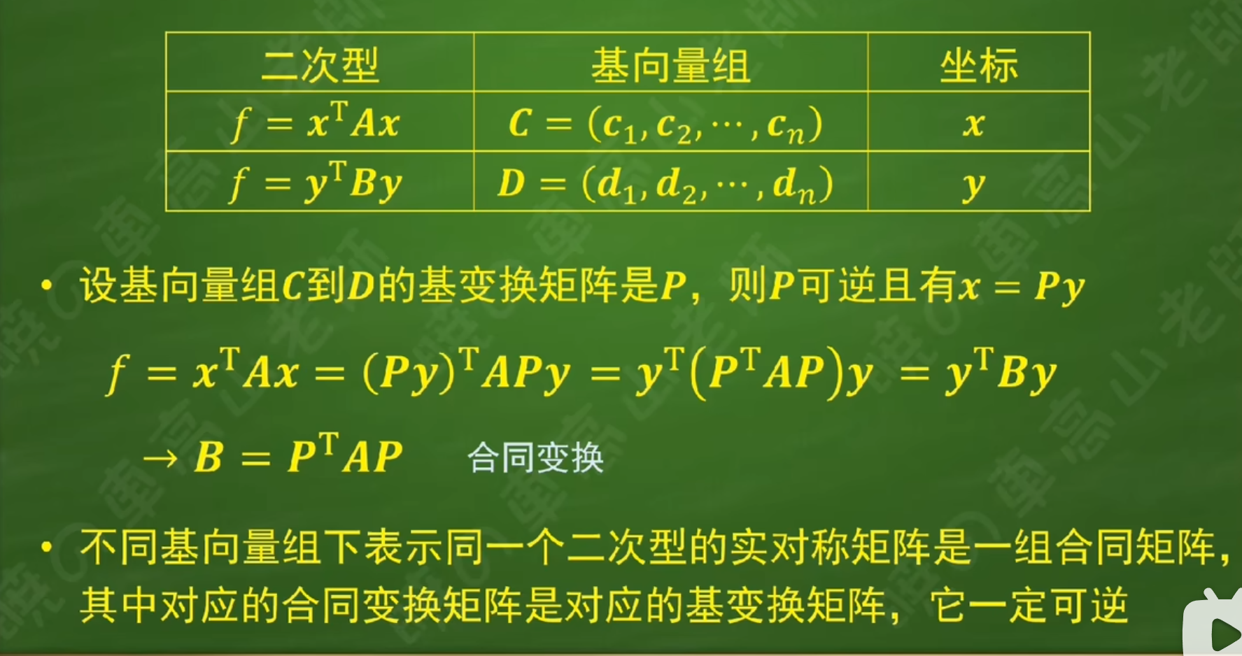
我们希望通过合同对角化（正交变换）将这个矩阵转化为对角矩阵，从而得到标准椭圆的形式。这样就可以得到长短轴。

假设矩阵 $A$ 的特征向量分别为 $v_1$ 和 $v_2$ ，则矩阵 $P$ 由这两个特征向量组成，且：

P = \begin{bmatrix} v_1 & v_2 \end{bmatrix}

如果我们使用矩阵 $P$ 进行坐标变换，即令新的坐标 $x'$ 为：

x' = P^{-1} x

那么，经过坐标变换后，二次型方程变为：

x'^T \Lambda x' = 1

其中 $\Lambda = \text{diag}(\lambda_1, \lambda_2)$ 是对角矩阵，包含了二次型的特征值。

\frac{x_1'^2}{\frac{1}{\sqrt{\lambda_1}}^2} + \frac{x_2'^2}{\frac{1}{\sqrt{\lambda_2}}^2} = 1

这意味着：

长轴的半长轴 $a = \frac{1}{\sqrt{\lambda_1}}$ ,
短轴的半长轴 $b = \frac{1}{\sqrt{\lambda_2}}$ .

为了对角化矩阵 $A$ ，我们首先求解其特征值和特征向量。特征值 $\lambda_1$ 和 $\lambda_2$ 是矩阵 $A$ 的解，满足以下特征方程：

\det(A - \lambda I) = 0

即：

\det\begin{bmatrix} a - \lambda & b \\ b & c - \lambda \end{bmatrix} = 0

计算行列式：

(a - \lambda)(c - \lambda) - b^2 = 0

展开后得到：

\lambda^2 - (a + c)\lambda + (ac - b^2) = 0

这个方程的解就是矩阵 ( A ) 的特征值 ( \lambda_1 ) 和 ( \lambda_2 )，分别为：

\lambda_1, \lambda_2 = \frac{(a + c) \pm \sqrt{(a + c)^2 - 4(ac - b^2)}}{2}

这两个特征值即为二次型的主轴方向上的系数，它们决定了椭圆的长短轴。

分布变换