前言
本次作业的内容是对上一次作业中的BVH遍历、射线三角形求交Möller-Trumbore算法进行迁移,以及在此基础上实现完整的 Path Tracing 算法。
请注意: 本次作业基于dalao的GAMES101作业框架 ,在Windows系统上实现。
函数迁移
Bounds3::IntersectP in Bounds3.hpp
本次作业中 cornell box 模型的墙壁和箱子某些三角形是平行于坐标平面的,会出现包围盒厚度为0的情况,因此求交要包含t_enter = t_exit 的情况。
1 2 3 4 5 6 7 8 9 10 11 12 13 14 15 16 17 18 19 20 21 22 23 24 25 26 27 28 29 30 31 32 33 34 35 36 37 38 39 40 inline bool Bounds3::IntersectP (const Ray& ray, const Vector3f& invDir, const std::array<int , 3 >& dirIsNeg) const float min_x = (pMin.x - ray.origin.x) * invDir[0 ]; float max_x = (pMax.x - ray.origin.x) * invDir[0 ]; float min_y = (pMin.y - ray.origin.y) * invDir[1 ]; float max_y = (pMax.y - ray.origin.y) * invDir[1 ]; float min_z = (pMin.z - ray.origin.z) * invDir[2 ]; float max_z = (pMax.z - ray.origin.z) * invDir[2 ]; if (dirIsNeg[0 ]) { std::swap (min_x, max_x); } if (dirIsNeg[1 ]) { std::swap (min_y, max_y); } if (dirIsNeg[2 ]) { std::swap (min_z, max_z); } float t_enter = std::max (min_x, std::max (min_y, min_z)); float t_exit = std::min (max_x, std::min (max_y, max_z)); if (t_enter <= t_exit && t_exit >= 0 ) { return true ; } else return false ; }
BVHAccel::getIntersection in BVH.cpp
1 2 3 4 5 6 7 8 9 10 11 12 13 14 15 16 17 18 19 20 Intersection BVHAccel::getIntersection (BVHBuildNode* node, const Ray& ray) const std::array<int , 3Ui64> dirIsNeg = { static_cast <int >(ray.direction.x < 0 ),static_cast <int >(ray.direction.y < 0 ),static_cast <int >(ray.direction.z < 0 ) };; if (node->bounds.IntersectP (ray, ray.direction_inv, dirIsNeg) == false ) { return Intersection{}; } if (node->left == nullptr && node->right == nullptr ) { return node->object->getIntersection (ray); } Intersection hit1 = getIntersection (node->left, ray); Intersection hit2 = getIntersection (node->right, ray); return hit1.distance < hit2.distance ? hit1 : hit2; }
Triangle::getIntersection in Triangle.hpp
1
2
3
4
5
6
7
8
9
10
11
12
13
14
15
16
17
18
19
20
21
22
23
24
25
26
27
28
29
30
31
32
33
34
35
36
37
38
39
40
41
42
inline Intersection Triangle::getIntersection (Ray ray) if (dotProduct (ray.direction, normal) > 0 ) { return Intersection{}; } Vector3f s = ray.origin - v0; Vector3f s1 = crossProduct (ray.direction, e2); Vector3f s2 = crossProduct (s, e1); float de = dotProduct (s1, e1); if (fabs (denominator) < EPSILON) { return Intersection{}; } float coefficient = 1.0f / denominator; float t = coefficient * dotProduct (s2, e2); float b1 = coefficient * dotProduct (s1, s); float b2 = coefficient * dotProduct (s2, ray.direction); float b0 = 1.0f - b1 - b2; if (t >= 0.0f && b0 >= 0.0f && b0 <= 1.0f && b1 >= 0.0f && b1 <= 1.0f && b2 >= 0.0f && b2 <= 1.0f ) { Intersection inter; inter.distance = t; inter.normal = normal; inter.coords = ray (t); inter.happened = true ; inter.m = m; inter.obj = this ; return inter; } else return Intersection{}; }
Path Tracing
L o ( p , ω 0 ) = L e ( p , ω 0 ) + ∫ Ω + L i ( p , ω i ) f r ( p , w i , w 0 ) ( n ⋅ ω i ) d w i \Large
_{Lo\left( p,\omega _0 \right) \ =\ L_e\left( p,\omega _0 \right) \ +\ \int\limits_{\varOmega +}^{}{L_i\left( p,\omega _i \right) f_r\left( p,w_i,w_0 \right) \left( n\cdot \omega _i \right) dw_i}}
L o ( p , ω 0 ) = L e ( p , ω 0 ) + Ω + ∫ L i ( p , ω i ) f r ( p , w i , w 0 ) ( n ⋅ ω i ) d w i
其中第一项表示物体本身的发出的光照强度,第二项的积分所包括的内容就是反射函数 Reflection Equation,即
L o ( p , ω 0 ) = ∫ Ω + L i ( p , ω i ) f r ( p , w i , w 0 ) cos θ i d w i \Large_{Lo\left( p,\omega _0 \right) \,\,=\,\,\int\limits_{\varOmega +}^{}{L_i\left( p,\omega _i \right) f_r\left( p,w_i,w_0 \right) \cos \theta _idw_i}}
L o ( p , ω 0 ) = Ω + ∫ L i ( p , ω i ) f r ( p , w i , w 0 ) c o s θ i d w i
L o ( p , ω 0 ) = ∫ A L i ( p , ω i ) f r ( p , w i , w 0 ) cos θ i cos θ i ′ ∥ x ′ − x ∥ 2 d A ( 从光源处采样 ) \Large
_{Lo\left( p,\omega _0 \right) \,\,
=\int\limits_A^{}{L_i\left( p,\omega _i \right) f_r\left( p,w_i,w_0 \right) \frac{\cos \theta _i\cos \theta _{i}^{\prime}}{\lVert x^{\prime}-x \rVert ^2}dA\left( \text{从光源处采样} \right)}}
L o ( p , ω 0 ) = A ∫ L i ( p , ω i ) f r ( p , w i , w 0 ) ∥ x ′ − x ∥ 2 c o s θ i c o s θ i ′ d A ( 从光源处采样 )
其中第一项是入射方向的Radiance,代表从单位立体角入射到单位面积上的光照强度。第二项就是双向反射分布函数BRDF(Bidirectional Reflectance Distribution Function) (只与材质有关 B R D F = M a t e r i a l BRDF = Material B R D F = M a t e r i a l
f r ( ω i → ω r ) = d L r ( ω r ) d E i ( ω i ) = d L r ( ω r ) L i ( ω i ) cos θ i d ω i [ 1 s r ] f_r\left( \omega _i\rightarrow \omega _r \right) =\frac{dL_r\left( \omega _r \right)}{dE_i\left( \omega _i \right)}=\frac{dL_r\left( \omega _r \right)}{L_i\left( \omega _i \right) \cos \theta _id\omega _i}\left[ \frac{1}{sr} \right]
f r ( ω i → ω r ) = d E i ( ω i ) d L r ( ω r ) = L i ( ω i ) cos θ i d ω i d L r ( ω r ) [ s r 1 ]
蒙特卡洛积分 Monte Carlo Intergration:
∫ f ( x ) d x = ∫ f ( x ) p ( x ) p ( x ) d x = E ( f ( x ) ) p ( x ) = 1 N ∑ i = 1 N f ( x i ) p ( x i ) ( 大数定律 ) \begin{aligned}
\int{f\left( x \right) dx=\int{\frac{f\left( x \right)}{p\left( x \right)}p\left( x \right) dx}}
=\frac{E\left( f\left( x \right) \right)}{p\left( x \right)}
=\frac{1}{N}\sum_{i=1}^N{\frac{f\left( x_i \right)}{p\left( x_i \right)}\left( \text{大数定律} \right)}\text{
}
\end{aligned}
∫ f ( x ) d x = ∫ p ( x ) f ( x ) p ( x ) d x = p ( x ) E ( f ( x ) ) = N 1 i = 1 ∑ N p ( x i ) f ( x i ) ( 大数定律 )
采样越多,方差越小
在这里的路径追踪中,我们根据渲染方程着色、利用蒙特卡洛估计离散化、 俄罗斯轮盘赌控制深度、 重复单次采样来降低方差和减少计算量、 从光源处采样来提高效率。
简要地说,就是根据光路可逆原理,从视线(viewpoint)发出一条光线到物体,再①从光源处采样,再追踪这个方向到物体的光线,如果没有遮挡就计算直接光照;②根据材质生成一条任意的wi,有物体相交就是间接光照,递归计算即可,无相交物体或到达光源时停止。
1 2 3 4 5 6 7 8 9 10 11 12 13 14 15 16 17 18 19 20 21 22 23 24 25 26 27 28 29 30 31 32 33 34 35 36 37 38 39 40 41 42 43 44 45 46 47 48 49 50 51 52 53 54 55 56 57 58 59 60 61 62 63 64 65 66 67 68 69 70 71 72 73 Vector3f Scene::castRay (const Ray& ray, int depth) const Intersection inter = intersect (ray); if (!inter.happened) { return Vector3f{ 0.0f , 0.0f , 0.0f }; } if (inter.m->hasEmission ()) { if (depth == 0 ) { return inter.m->getEmission (); } else return Vector3f{ 0.0f , 0.0f , 0.0f }; } Vector3f view_dir = ray.direction; Vector3f normal = inter.normal.normalized (); Vector3f position = inter.coords; Vector3f L_dir = { 0.0f ,0.0f ,0.0f }, L_indir = {0.0f , 0.0f , 0.0f }; Intersection inter_light; float pdf_light; sampleLight (inter_light, pdf_light); Vector3f normal_light = normalize (inter_light.normal); Vector3f position_light = inter_light.coords; Vector3f light_dir = (position - position_light).normalized (); float distanceToLight = (position-position_light).norm (); float distanceToLight2 = dotProduct (position - position_light, position - position_light); Ray lightToObj (position_light, light_dir) ; Intersection inter_lightToObj = intersect (lightToObj); float distanceToObj = inter_lightToObj.distance; if (inter_lightToObj.happened && distanceToObj - distanceToLight > -EPSILON) { Vector3f f_r = inter.m->eval (view_dir, -light_dir, normal); float cos_theta = dotProduct (-light_dir, normal); float cos_theta_l = dotProduct (light_dir, normal_light); L_dir = inter_light.emit*f_r * cos_theta * cos_theta_l / (pdf_light * distanceToLight2); } float ksi = get_random_float (); if (ksi < RussianRoulette) { Vector3f obj_dir = inter.m->sample (view_dir, normal); Ray ObjToScene (position, obj_dir) ; Intersection inter_ObjToScene = intersect (ObjToScene); if (inter_ObjToScene.happened && !inter_ObjToScene.m->hasEmission ()) { Vector3f f_r = inter.m->eval (view_dir, obj_dir, normal); float cos_theta = dotProduct (obj_dir, normal); float pdf_hemi = inter.m->pdf (view_dir, obj_dir, normal); if (pdf_hemi > EPSILON) { L_indir = f_r * castRay (ObjToScene, depth + 1 ) * cos_theta / (pdf_hemi * RussianRoulette); } } } return L_dir + L_indir; }
多线程
在这里运用C++11中的thread可以轻松地分像素进行并行渲染。
1 2 3 4 5 6 7 8 9 10 11 12 13 14 15 16 17 18 19 20 21 22 23 24 25 26 27 28 29 30 31 32 33 34 35 36 37 38 39 40 int spp = 256 ; std::cout << "SPP: " << spp << "\n" ; const int thread_cnt = 8 ;int finished_thread = 0 ;int finished_width = 0 ;std::mutex mtx; printf ("%d %d\n" , scene.height, scene.width);auto multiThreadCastRay = [&](uint32_t y_min, uint32_t y_max){ printf ("start %d %d\n" , y_min, y_max); for (uint32_t j = y_min; j <= y_max; ++j) { for (uint32_t i = 0 ; i < scene.width; ++i) { float x = (2 * (i + 0.5 ) / (float )scene.width - 1 ) * imageAspectRatio * scale; float y = (1 - 2 * (j + 0.5 ) / (float )scene.height) * scale; Vector3f dir = normalize (Vector3f (-x, y, 1 )); for (int k = 0 ; k < spp; k++) { framebuffer[scene.width * j + i] += scene.castRay (Ray (eye_pos, dir), 0 ) / spp; } } mtx.lock (); UpdateProgress (++finished_width * 1.0 / scene.width); mtx.unlock (); } printf ("ok %d %d\n" , y_min, y_max); }; int block = scene.height / thread_cnt + (scene.height % thread_cnt != 0 );std::thread th[thread_cnt]; for (int i = 0 ; i < thread_cnt; i++) { th[i] = std::thread (multiThreadCastRay, i * block, std::min ((i + 1 ) * block - 1 , scene.height)); } for (int i = 0 ; i < thread_cnt; i++) th[i].join ();UpdateProgress (1.0 );
加速及优化
将Debug更换为Release
Debug 是调试版本,包含调试信息,不优化代码,便于程序员调试;
Release 是发布版本,不包含调试信息,对代码进行优化,便于用户使用。
在图形学中,常常需要进行大量的计算和像素的处理。更换为Release可以大幅提高编译效率,进行更加顺利的测试。
get_random_float() in global.hpp
global.hpp下的get_random_float()随机数生成函数存在问题,它会导致在重复调用该函数时,返回同一个值。
1 2 3 4 5 6 7 8 9 static std::random_device dev;static std::mt19937 rng (dev()) static std::uniform_real_distribution<float > dist (0.f , 1.f ) inline float get_random_float () return dist (rng); }
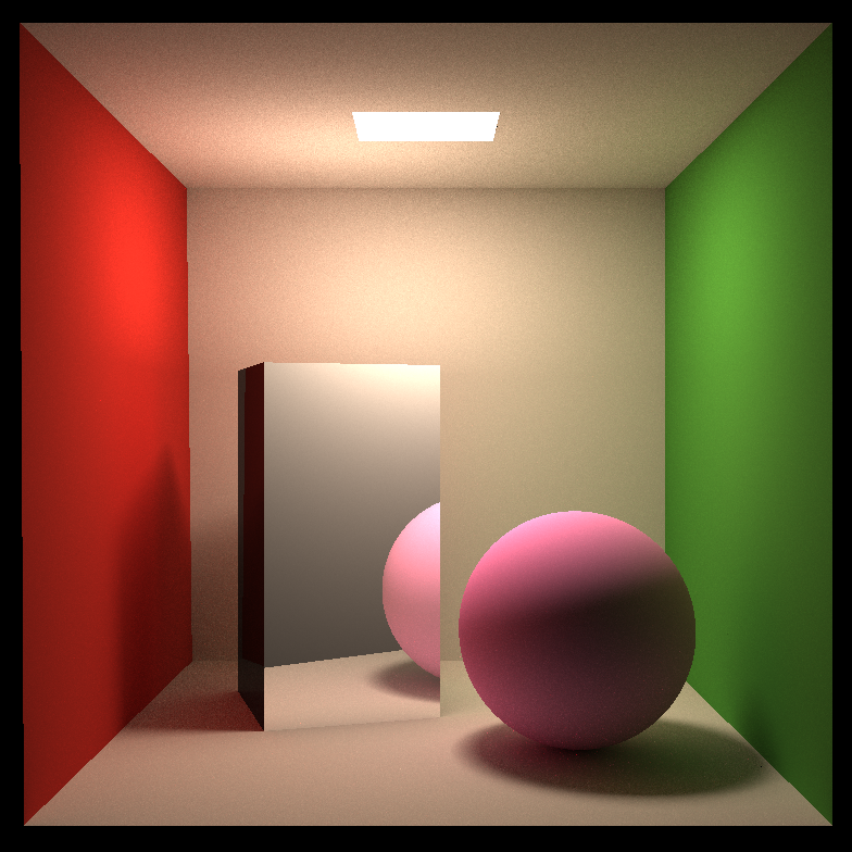
白色噪点
原因应该是pdf接近于0时,除以它计算得到的颜色会偏向极限值,体现在图上也就是白色
Microfacet微平面理论
LearnOpenGL
BRDF = Material
f r = k d f l a m b e r t + k s f c o o k − t o r r a n c e \large
f_r=k_df_{lambert}+k_sf_{cook-torrance}
f r = k d f l a m b e r t + k s f c o o k − t o r r a n c e
其中:
k d kd k d k s ks k s k d + k s = 1 kd+ks=1 k d + k s = 1
f l a m b e r t f_{lambert} f l a m b e r t f c o o k − t o r r a n c e f_{cook-torrance} f c o o k − t o r r a n c e
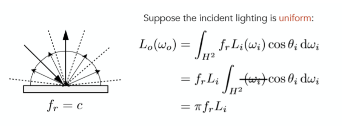
Lambertian漫反射 L i = L o L_{i}=L_{o} L i = L o f r = 1 π f_r=\frac{1}{\pi} f r = π 1
f l a m b e r t = ρ π \large
f_{lambert}=\frac{\rho}{\pi}
f l a m b e r t = π ρ
其中ρ {\rho} ρ
Cook-Torrance BRDF
f ( l , v ) = D ( h ) F ( v , h ) G ( l , v , h ) 4 ( n ⋅ l ) ( n ⋅ v ) \large
f\left( l,v \right) =\frac{D\left( h \right) F\left( v,h \right) G\left( l,v,h \right)}{4\left( n\cdot l \right) \left( n\cdot v \right)}
f ( l , v ) = 4 ( n ⋅ l ) ( n ⋅ v ) D ( h ) F ( v , h ) G ( l , v , h )
其中:
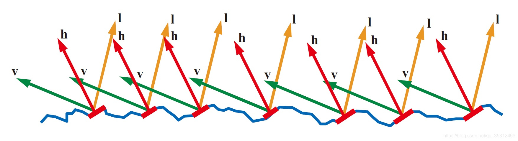
光照方向L,观察方向V, 微观法线/中间向量H,宏观向量N D(h):法线分布函数(Normal Distribution Function) ,描述微面元法线分布的概率,即正确朝向的法线的浓度。即具有正确朝向,能够将来自l的光反射到v的表面点的相对于表面面积的浓度。F(v,h):菲涅尔方程(Fresnel Equation) ,描述不同的表面角下表面所发射的光线所占的比率。G(l,v,h):几何函数(Geometry Function) ,描述微平面自成阴影的属性,即m=h的未被遮蔽的表面点的百分比。4(n*l)(n*v):校正因子(Correctionfactor) ,作为微观几何的局部空间和整个宏观表面的局部空间之间变换的微平面量的校正。
微表面模型需要用到的参数 :
V V V I I I m = h m=h m = h V V V I I I N N N α {\alpha} α
D(h):法线分布函数(Normal Distribution Function)
各项同性NDF
GGX(Trowbridge-Reitz)分布
α = R o u g h n e s s 2 \alpha =Roughness^2
α = R o u g h n e s s 2
D G G X ( m ) = α 2 π ( ( n ⋅ m ) 2 ( α 2 − 1 ) + 1 ) 2 D_{GGX}\left( \mathbf{m} \right) =\frac{\alpha ^2}{\pi \left( \left( \mathbf{n}\cdot \mathbf{m} \right) ^2\left( \alpha ^2-1 \right) +1 \right) ^2}
D G G X ( m ) = π ( ( n ⋅ m ) 2 ( α 2 − 1 ) + 1 ) 2 α 2
1
2
3
4
5
6
7
8
9
10
11
12
Vector3f D_GGXT (Vector3f N,Vector3f H,float rough) float a = rough * rough; float a2 = a * a; float NdotH = std::max (dotProduct (N, H), 0.0f ); float NdotH2 = NdotH * NdotH; float denom = (NdotH2 * (a2 - 1.0f ) + 1.0f ); denom = denom * denom; return a2 * MY_INV_PI * std::max (denom,0.0000001f ); }
各项异性NDF
Anisotropic GGX分布
D G G X a n i s o ( m ) = 1 π α x α y 1 ( ( t ⋅ m ) α x 2 + ( b ⋅ m ) α y 2 + ( n ⋅ m ) 2 ) 2 D_{GGXaniso}\left( \mathbf{m} \right) =\frac{1}{\pi \alpha _x\alpha _y}\frac{1}{\left( \frac{\left( \mathbf{t}\cdot \mathbf{m} \right)}{\alpha _{x}^{2}}+\frac{\left( \mathbf{b}\cdot \mathbf{m} \right)}{\alpha _{y}^{2}}+\left( \mathbf{n}\cdot \mathbf{m} \right) ^2 \right) ^2}
D G G X a n i s o ( m ) = π α x α y 1 ( α x 2 ( t ⋅ m ) + α y 2 ( b ⋅ m ) + ( n ⋅ m ) 2 ) 2 1
需要注意的是,将法线贴图与各向异性BRDF组合时,重要的是要确保法线贴图扰动(perturbs)切线和副切线矢量以及法线。
F(v,h):菲涅尔方程(Fresnel Equation)
v v v
Schlick Fresnel近似
F S c h l i c k ( v , h ) = F 0 + ( 1 − F 0 ) ( 1 − ( v ⋅ h ) ) 5 F_{Schlick}\left( \mathbf{v,h} \right) =F_0+\left( 1-F_0 \right) \left( 1-\left( v\cdot h \right) \right) ^5
F S c h l i c k ( v , h ) = F 0 + ( 1 − F 0 ) ( 1 − ( v ⋅ h ) ) 5
1
2
3
4
5
float F_Schlick (Vector3f V, Vector3f H,Vector3f F0) float cos_theta = std::max (dotProduct (V, H), 0.0f ); return F0 + (1.0f - F0) * std::pow ((1 - cos_theta), 5 ); }
G(l,v,h):几何函数(Geometry Function)
通常,除了近掠射角或非常粗糙的表面,几何函数对BRDF的形状影响相对较小,但对于BRDF保持能量守恒而言,几何函数至关重要。
在部分游戏引擎和文献中,几何函数G(l,v,h)和分母中的校正因子4(n·l)(n·v)会合并为可见性项(The
几何函数与法线分布函数作为Microfacet Specular BRDF中的重要两项,两者之间具有紧密的联系
V ( v , l ) = G ( l , v , h ) 4 ( n ⋅ l ) ( n ⋅ v ) \large
V\left( \mathbf{v,l} \right) =\frac{G\left( \mathbf{l,v,h} \right)}{4\left( \mathbf{n}\cdot \mathbf{l} \right) \left( \mathbf{n}\cdot \mathbf{v} \right)}
V ( v , l ) = 4 ( n ⋅ l ) ( n ⋅ v ) G ( l , v , h )
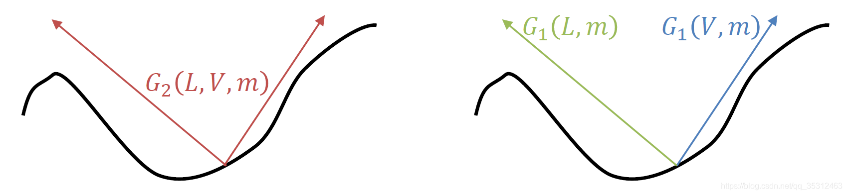
几何函数具有两种主要形式:G1和G2,其中:
G1为微平面在单个方向(光照方向L或观察方向V)上可见比例,一般代表遮蔽函数(masking
G2为微平面在光照方向L和观察方向V两个方向上可见比例,一般代表联合遮蔽阴影函数(joint masking-shadowing
默认情况下,microfacet BRDF中使用的几何函数代指G2
G 2 ( l , v ) 4 ∣ n ⋅ l ∣ ∣ n ⋅ v ∣ ≈ 0.5 l e r p ( 2 ∣ n ⋅ l ∣ ∣ n ⋅ v ∣ , ∣ n ⋅ l ∣ + ∣ n ⋅ v ∣ , α ) \frac{G_2\left( \mathbf{l,v} \right)}{4\left| \mathbf{n}\cdot \left. \mathbf{l} \right|\left| \left. \mathbf{n}\cdot \mathbf{v} \right| \right. \right.}\approx \frac{0.5}{lerp\left( 2\left| \left. \mathbf{n}\cdot \mathbf{l} \right|\left| \right. \left. \mathbf{n}\cdot \mathbf{v} \right|,\left| \left. \mathbf{n}\cdot \mathbf{l} \right|+\left| \left. \mathbf{n}\cdot \mathbf{v} \right|,\alpha \right. \right. \right. \right)}
4 ∣ n ⋅ l ∣ ∣ n ⋅ v ∣ G 2 ( l , v ) ≈ l e r p ( 2 ∣ n ⋅ l ∣ ∣ n ⋅ v ∣ , ∣ n ⋅ l ∣ + ∣ n ⋅ v ∣ , α ) 0 . 5
1 2 3 4 5 6 7 8 9 10 11 12 float Visibility (Vector3f V,Vector3f L,Vector3f N, float rough) float NdotV = std::max (dotProduct (N, V), 0.0f ); float NdotL = std::max (dotProduct (N, L), 0.0f ); float f = rough + 1.0 ; float k = f * f * 0.125 ; float ggxV = 1.0 / (NdotV * (1.0 - k) + k); float ggxL = 1.0 / (NdotL * (1.0 - k) + k); return ggxV * ggxL * 0.25 ; }
计算误差导致的交点偏离问题
1 2 3 4 5 6 7 8 9 10 11 12 13 14 15 16 17 18 19 20 21 22 23 Intersection getIntersection (Ray ray) { Intersection result; result.happened = false ; Vector3f L = ray.origin - center; float a = dotProduct (ray.direction, ray.direction); float b = 2 * dotProduct (ray.direction, L); float c = dotProduct (L, L) - radius2; float t0, t1; if (!solveQuadratic (a, b, c, t0, t1)) return result; if (t0 < 0 ) t0 = t1; if (t0 < 0 ) return result; if (t0 > 0.5 ) { result.happened = true ; result.coords = Vector3f (ray.origin + ray.direction * t0); result.normal = normalize (Vector3f (result.coords - center)); result.m = this ->m; result.obj = this ; result.distance = t0; } return result; }
总结:
参考资料:GAMES101作业7-路径追踪实现过程&代码框架超全解读 图形学入门笔记3:Path Tracing-Games101作业7 Games101 作业7 绕坑引路 (Windows) 【GAMES101】作业7 常见问题避坑